Background

In the era of complex engineering systems, computational models play a central role in systems design and analysis. A popular class of stochastic computational models are surrogate models, which are also often known as metamodels or response surfaces (depending on the research community and the interpretation). Surrogate models are purely mathematical models (i.e., not derived from the system physics) that are used to provide a tractable and inexpensive approximation of the actual system behavior. They are commonly used as an alternative to expensive computational simulations (e.g., CFD) or to the lack of a physical model in the case of experiment-derived data (e.g., creation and testing of new metallic alloys ). Surrogate models are generally expected to provide a low fidelity representation of the actual system behavior.
While a suitable surrogate model can be selected intuitively (experience-based selection), guided by an understanding of the data characteristics and/or the application constraints, the development of general guidelines might not be practical due to the diversity of system behavior among design applications. Only a few candidate surrogate model forms (or modeling methods), with which the user is well acquainted, are generally considered; thereby, the user often fails to exploit the large and fast-growing pool of surrogate models in the literature.
Objective/Goals of our research
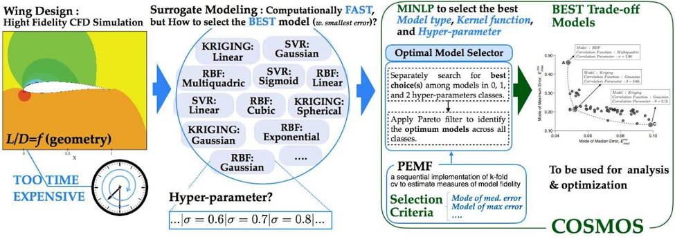
COSMOS is an automated model selection technique that works on all three levels of surrogate modeling: model type, basis function (or kernel / correlation function), and hyperparameter value. COSMOS examines all three levels to determine the surrogate with the least error. The goal of COSMOS is to provide researchers with a robust method for surrogate model selection.
Our Approach/Methodology
COSMOS determines the model type, basis function and hyperparameter value that minimize the error in the surrogate model. That error is measured by PEMF, a measure that is something like an advanced cross-validation. To find the PEMF error, a model is trained with only a fraction of the data. The remaining points are compared to the trained model, and error is computed. This process is repeated multiple times, increasing the fraction of data used for training each time, and noting the error at each fraction. The error in the model when all data is used can be predicted by plotting error vs. training fraction and extrapolating. This is a simplification, PEMF is actually a statistical measure of error. In fact one can consider a median PEMF error or (for applications where safety is critical) a maximum PEMF error — both were considered in this research. Interested readers should refer to “Predictive quantification of surrogate model fidelity based on modal variations with sample density” by Mehmani et. al. for more information on PEMF.
Findings till date/Conclusion
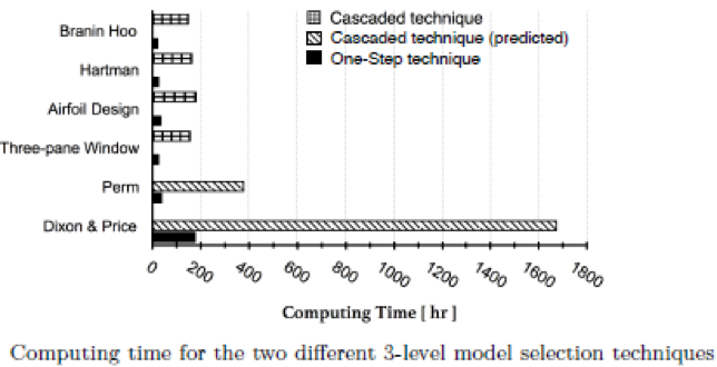
In order to find the model with the lowest PEMF error, one could use a cascaded approach wherein each model and basis function combination checked, but a “one-step” method was found to be faster. An optimization problem is formulated in which the three levels of surrogate modeling are variables. Standard optimization techniques are then applied to minimize the error in the surrogate model. A number of sample problems were solved with both techniques; the computing time results are shown below.

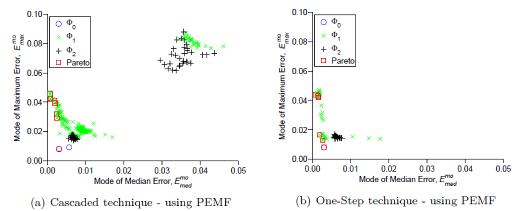
All models exhibited different performances for the different test problems. Shown below is a plot of the median and maximum error trade-off for the Airfoil design problem. It is easy to see that some models exhibit much better performance, and that the one-step technique produces better models.

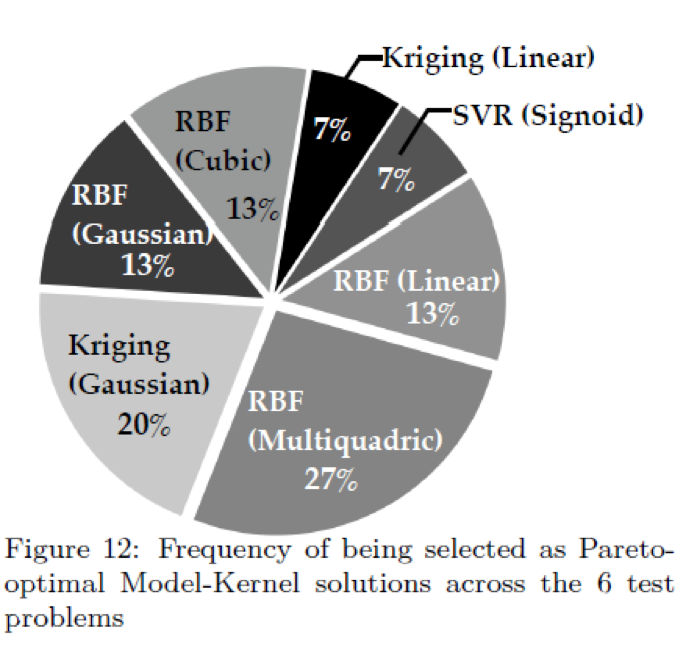
Across all the test problems, no one model was dominant. The plot below shows the relative frequency that a surrogate model had the least error.

Future work for COSMOS will focus on improving efficiency of the algorithm and applying it to difficult to solve design problems.